Data

A simple API for importing and preparing data for use. Mostly manipulates numpy arrays to generate profiles and sections

We will be treating 2D arrays as rasters. Basically load any .csv, .txt or other file into a numpy array as you would normally. Each entry should be the height data for it’s respective pixel.

Let’s try out the simplest method, a text file containing an (M,N) array compatible with Numpy. If you’d like to try your own data, simply change the file below and the loading function (e.g. if you have a .csv just change the delimeter in the np.loadtxt() call).

file = 'BYGS008_top_segment_500samp_10cm_interp089.txt'
image = np.loadtxt(file)

Let’s have a look at the image

plt.imshow(image)
plt.show()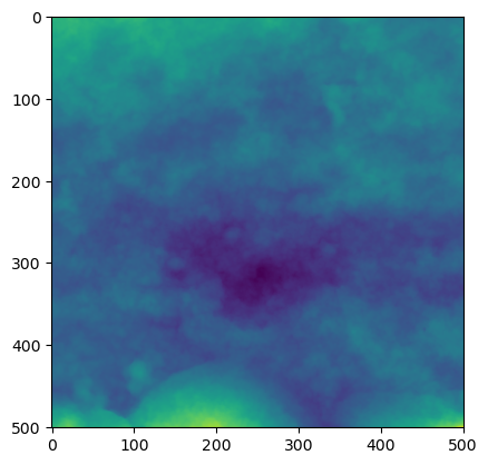

image.shape

(501, 501)

It can be very useful to study how roughness parameters change with regards to their orientation. The following function helps produce a range of profiles rotating around the central point of the image or array

---

source

gen_rot_prof

 gen_rot_prof (array, deg=180, increment=1)

Generates an array of rotational profiles through to deg, in even increments of increment. Uses OpenCV and Imutils to rotate the array around the center of the array/raster/image, extracts the middle row.

	Type	Default	Details
array			2D array of height values
deg	int	180	Number of degrees to rotate through, i.e 180 gives full 360 rotation
increment	int	1	deg/increment = number of evenly spaced profiles to calculate.

Numpy likes the data in various forms for linear algebra, here is a helper to convert an (M,N) matrix into a (n,(X,Y,Z)) matrix.

---

source

image2xyz

 image2xyz (im)

Converts 2D (m,n) image/array to xyz coordinates. Used for plane levelling

---

source

xyz2image

 xyz2image (xyz)

Helper to convert back from xyz (n,3) arrays to (M,N) image/matrices

	Details
xyz	(n,3) shape array

im_xyz = image2xyz(image)
im_xyz[:5]

array([[ 0.        ,  0.        , -0.89188266],
       [ 1.        ,  0.        , -0.8919338 ],
       [ 2.        ,  0.        , -0.89193225],
       [ 3.        ,  0.        , -0.89193505],
       [ 4.        ,  0.        , -0.89192402]])

Levelling and Form Removal

In order to perform roughness calculations it is recommended to level the data and remove the underlying form.This produces a S-F surface from the primary surface if we are using Standards terms. Because surfaces are always digitized and discretized in some way, the actual surface has to be modelled using some function. ISO software standards recommend using a Bicubic spline to remove the form. Because the function is an assumption, the user should choose their function based on their scientific knowledge of the surface and the goals of their research. Multiple functions can be tested and the results observed. Here I provide a least-squares solution to the problem, computing the results in the same shape as the original image and subtract them.

With the underlying form modeled, the funciton can be sampled from to generate a larger number of samples.

---

source

remove_form

 remove_form (im, degree=3, return_form=False)

Remove the form of the raster by fitting a polynomial of specified degree and subtracting it.

	Type	Default	Details
im			2D Numpy array or array like
degree	int	3	Polynomial degree to remove
return_form	bool	False	Return the form/computed polynomial values instead of removing them from im

---

source

plane_level

 plane_level (im, norm=True, return_form=False)

Level an (m,n) array by computing the best fit plane and subtracting the results. Thin wrapper around remove_form with degree = 1.

	Type	Default	Details
im			Numpy array or array like
norm	bool	True	Normalize the data by subtracting the mean
return_form	bool	False

w = np.array([[1,1,1],[0,0,0],[-1,-1,-1]])
u = np.array([[1,0,-1]]*3)
test_close(plane_level(w), np.zeros(w.shape))
test_close(plane_level(u), np.zeros(u.shape))
test_fail(plane_level, kwargs = dict(xyz=np.array([1])))
test_fail(plane_level, kwargs = dict(xyz=np.array([[1,1]])))

fig = plt.figure()
ax = fig.add_subplot(1, 2, 1)
imgplot = plt.imshow(plane_level(image))
ax.set_title('Levelled image')
ax = fig.add_subplot(1, 2, 2)
imgplot = plt.imshow(plane_level(image, return_form = True))
ax.set_title('Levelling plane')

Text(0.5, 1.0, 'Levelling plane')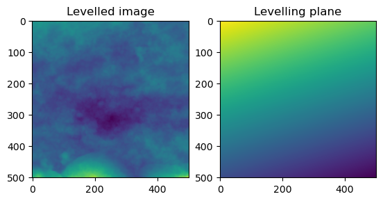

image_f = remove_form(plane_level(image))
image_form = remove_form(plane_level(image), return_form = True)

fig = plt.figure()
ax = fig.add_subplot(1, 2, 1)
imgplot = plt.imshow(image_f)
ax.set_title('Formless Image')
ax = fig.add_subplot(1, 2, 2)
imgplot = plt.imshow(image_form)
ax.set_title('Polynomial')

Text(0.5, 1.0, 'Polynomial')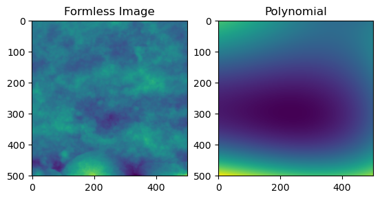

Noise and smoothing

Similarly, it is recommended to remove noise and attenuate high frequency features. We achieve this through the use of a gaussian filter.

---

source

smooth_image

 smooth_image (array, sigma=None, alpha=None, cutoff=None, axis=None,
               **kwargs)

*Removes high frequency/wavelength features (‘noise’) by applying a gaussian filter on the image. Thin wrapper of scipy.ndimage.gaussian_filter.

If all sigma,alpha,cutoff = None, sigma defaults to (np.sqrt(np.log(2)/np.pi)) * cutoff

If sigma is not none, sigma takes priority over any alpha or cutoff provided.

Refer to ISO 11562:1997 for reasoning behind alpha and cutoff.*

	Type	Default	Details
array			Numpy array or array like
sigma	NoneType	None	Standard deviation for gaussian kernel Useful for determining the wavelength of the low pass filter.
alpha	NoneType	None	Used in gaussian weighting function, defaults to np.sqrt(np.log(2)/np.pi)
cutoff	NoneType	None	Cutoff wavelength, defaults to 1
axis	NoneType	None	Axis along which to apply filter
kwargs

image_f_s = smooth_image(image_f,cutoff=1)

fig = plt.figure()
ax = fig.add_subplot(1, 2, 1)
imgplot = plt.imshow(image_f_s)
ax.set_title('Sigma = 1')
ax = fig.add_subplot(1, 2, 2)
imgplot = plt.imshow(smooth_image(image_f,cutoff=10))
ax.set_title('Sigma = 10')

Text(0.5, 1.0, 'Sigma = 10')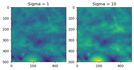

Sections

It can be useful to study subsections of surfaces. The following helpers assist with this process. Otherwise, normal manipulation of numpy arrays is always possible.

---

source

gen_sections

 gen_sections (image, how='square', number=100)

Generates sections of the array/image, either in square, horizontal, or vertical sections. Useful for studying the change of parameters over the surface. Mostly wraps around np.hsplit and np.vsplit. Note, if ‘number’ does not divide into the array evenly, the bottom/side remains will not be included.

	Type	Default	Details
image			2D array (or arraylike) of height values
how	str	square	How to subdivide the array, options are: ‘square’, ‘row’, ‘column’
number	int	100	Number of sections to produce

a_10000 = np.arange(100*100).reshape(100,100)
test_eq(gen_sections(a_10000)[0],a_10000[:10,:10])

a_523 = np.arange(523*523).reshape(523,523)
a_520 = np.arange(520*520).reshape(520,520)
test_eq(gen_sections(a_523).shape,gen_sections(a_520).shape)

test_sections = np.load('example_sections.npy')
test_sections.shape

(100, 50, 50)

image_sections =  gen_sections(image)

Now, because we’ve applied all of our preprocessing steps to the original image. We can export it for use later. We should also save our profiles and sections. The sections should be in .npy format because they are 3D.

np.savetxt('example.txt', image_f_s)
np.savetxt('example_profiles.txt', gen_rot_prof(image_f_s))
np.save('example_sections.npy', image_sections)

And we can load them back in just to check.

profiles = np.loadtxt('example_profiles.txt')
plt.imshow(profiles)
plt.show()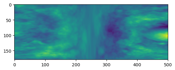

Utilities

Various useful functions which are used elsewhere

---

source

compute_parameters

 compute_parameters (array, parameter_list:list, valid_module=None,
                     to_df:bool=False, **kwargs)

Computes a set of parameters for a given array, provide a list of parameters (as strings of their respective functions e.g. [‘Ra’,‘Rms’]) and a module to verify against (might require some module aliasing, see CLI notebook for example use). Returns a list of results or a dataframe.

	Type	Default	Details
array			Input array to be calculate parameters on
parameter_list	list		List of parameters to calculate as strings
valid_module	NoneType	None	module to generate functions from, used to check user input, see rough.cli:rough
to_df	bool	False	Return the parameters as a pandas dataframe, with columns set as the parameter names
kwargs

---

source

distance_matrix

 distance_matrix (shape:tuple, center:(<class'int'>,<class'int'>)=None,
                  sections=False)

*Returns a (m,n) matrix containing distance values from center coordinates.

if Sections = True. Returns (x,m,n) where x is the number of input sections.*

	Type	Default	Details
shape	tuple		Shape of array, used to calculate center if not given
center	(<class ‘int’>, <class ‘int’>)	None	Central point from which to calculate distances, if None, defaults to x//2, y//2
sections	bool	False	If True, takes the first element of shape as the number of stack in image

a25 = np.arange(25).reshape(5,5)

a25.shape

(5, 5)

a25t = np.tile(a25,(5,5,5))

test_eq(a25t[0],a25t[4])

test_shape = (101,101)
#eps = 1e-05
test_eq(distance_matrix(test_shape), np.rot90(distance_matrix(test_shape)))
test_eq(distance_matrix(test_shape), np.flipud(distance_matrix(test_shape)))
test_eq(distance_matrix(test_shape), np.fliplr(distance_matrix(test_shape)))

test_ne(distance_matrix(test_shape), np.zeros(test_shape))
test_ne(distance_matrix(test_shape), np.ones(test_shape))

---

source

normalize

 normalize (im, axis=1, how='center', feature_range=None)

*Normalize the input array along given axis. Typically used to ‘center’ rows/columns/areas in order to calculate parameters. how can be: - ‘center’: Subtract the mean from the array along the axis, - ‘l1’ - ‘l2’ - ‘standardize’ : Subtract the mean and divide by the standard deviation along given axis - ‘minmax’ : ‘standardize’ within ‘feature_range’. See use in Sal

Mostly a reimplementation of scalers from sklearn with explicit formulation.*

	Type	Default	Details
im			Array or stack of array to normalize
axis	int	1	Axis along which to normalize
how	str	center	normalization method: ‘center’, ‘standardize’, ‘minmax’
feature_range	NoneType	None	Tuple containing the feature range for minmax

#For testing normalize
from sklearn.preprocessing import MinMaxScaler

a_400 =np.arange(-200,200).reshape(-1,1)
a_rand = np.random.randint(-1000,1000,1000).reshape(-1,1)
scaler = MinMaxScaler((-1,1))

test_eq((a_400 - np.mean(a_400,axis = 0,keepdims = True)), normalize(a_400, axis = 0, how = 'center'))
test_eq((a_rand - np.mean(a_rand,axis = 0, keepdims = True)), normalize(a_rand,axis = 0, how = 'center'))

test_close(scaler.fit_transform(a_400),  normalize(a_400,axis = 0, how = 'minmax'), eps = 1e-10)
test_close(scaler.fit_transform(a_rand), normalize(a_rand,axis = 0, how = 'minmax'), eps = 1e-10)

image_f_s.shape

(501, 501)

from scipy.signal import correlate

cor_result = correlate(image_f_s, image_f_s,mode='same')
plt.imshow(cor_result)
plt.show()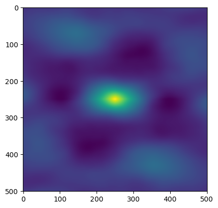

correlate(np.ones((3,3)), np.ones((3,3)), mode = 'same')

array([[4., 6., 4.],
       [6., 9., 6.],
       [4., 6., 4.]])

rand_arr = np.random.rand(501,501)
rand_cor = correlate(rand_arr,rand_arr,mode='same')
plt.imshow(rand_cor)
plt.show()

(np.amax(rand_cor),np.amin(rand_cor),np.ptp(rand_cor))

(83755.5666617089, 15717.948579544685, 68037.61808216422)

rand_ncor = normalize(rand_cor,axis = None, how= 'minmax')

(np.amax(rand_ncor),np.amin(rand_ncor),np.ptp(rand_ncor))

(1.0, -1.0, 2.0)

plt.imshow(rand_ncor)
plt.show()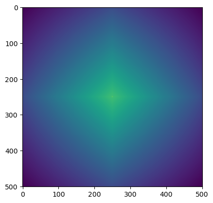

rand_dist = distance_matrix(rand_ncor.shape)

rand_where = np.where(rand_ncor <= 0.2, rand_dist, np.NaN)
np.nanmin(rand_where)

36.76955262170047

x = np.linspace(0, 20)
y = np.sin(x)
sin_wave = np.broadcast_to(y,(50,50))

plt.imshow(sin_wave)
plt.show()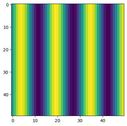

plt.imshow(sin_wave.T)
plt.show()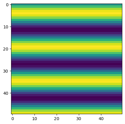

sin_cor = correlate(sin_wave,sin_wave,mode='same')
plt.imshow(sin_cor)
plt.show()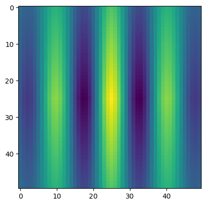

ncor_sin = normalize(sin_cor, axis = None, how = 'minmax')
plt.imshow(ncor_sin)
plt.show()

ncor_sin_2 = np.where(ncor_sin <=0.2, ncor_sin, np.NaN)
plt.imshow(ncor_sin_2)
plt.show()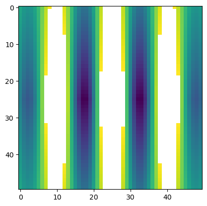

sint_cor = correlate(sin_wave.T,sin_wave.T,mode='same')
plt.imshow(sint_cor)
plt.show()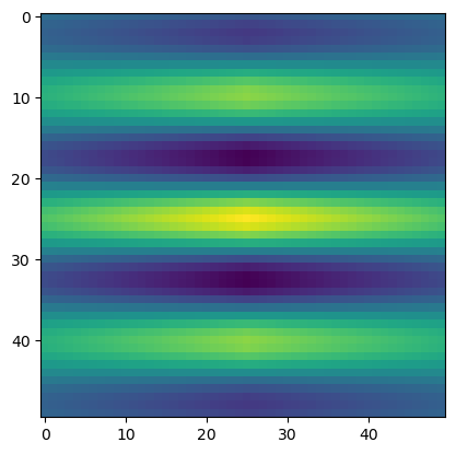

sin_cor[-1,-1]

-302.59161125378563

(np.ptp(cor_result),np.max(cor_result),np.min(cor_result))

(0.12309696498814524, 0.10140944660491391, -0.021687518383231318)